Kuhn-Tucker Conditions and Contact Formulation

Preface #

The general formulation of contact problems aligns closely with the structure of the Kuhn-Tucker (KT) conditions . So, I take this opportunity to revisit the derivation of the KT conditions in order to deepen my understanding of both topics.

Kuhn-Tucker Conditions #

In this section, we will provide a detailed trace of deriving the well-known Kuhn-Tucker conditions, which serve as the ‘first-order necessary conditions’ for extremum.

Unconstrained Optimization of Univariate Functions #

$$\min\ f(x),\quad -\infty\leq x\leq\infty$$

The necessary condition for a global minimum is given by: $$\left.\frac{\mathrm{d}f(x)}{\mathrm{d}x}\right|_{x=x^\ast}=0, \tag{1}$$ and the sufficient condition is $$\left.\frac{\mathrm{d}^2f(x)}{\mathrm{d}x^2}\right|_{x=x^\ast}>0, \tag{2}$$ which indicates the function considered is convex.

Unconstrained Optimization of Multivariate Functions #

$$\min\ f(\pmb{x}),\quad \pmb{x}=\left\{x_1,x_2,\,\cdots,x_n\right\}^\mathrm{T},\ -\infty\leq x_i\leq\infty$$

The directional derivative of $f(\pmb{x})$ is defined as $\nabla_{\pmb{v}}f=\nabla f\cdot\pmb{v}$, where $$\nabla f=\left\{\frac{\partial f}{\partial x_1},\frac{\partial f}{\partial x_2},\,\cdots,\frac{\partial f}{\partial x_n}\right\}^\mathrm{T} \tag{3}$$ is called the gradient of function $f(\pmb{x})$.

The necessary condition for a global minimum in this case is given by $$\nabla f(\pmb{x}^\ast)=\boldsymbol{0}, \tag{4}$$ while the sufficient condition is stated as the Hessian Matrix $\mathcal{H}$ should be positive definite , i.e., we have $\pmb{y}^\mathrm{T}\mathcal{H}\pmb{y}>0$ for all $\pmb{y}\neq\pmb{0}$. Here the Hessian Matrix takes the form: $$\mathcal{H}=\nabla^2 f=\left[\frac{\partial^2 f}{\partial x_i\partial x_j}\right].$$

Equality Constrained Optimization of Multivariate Functions #

\begin{align} \min\quad &f(\pmb{x}),\quad \pmb{x}=\left\{x_1,x_2,\,\cdots,x_n\right\}^\mathrm{T},\\ \mathrm{s.t.}\quad &h_j(\pmb{x})=0,\quad j=1,2,\,\cdots,m. \end{align}

For this kind of optimization problem, we use the Lagrange Multiplier method to incorporate the original constraint terms into the objective function, thus yielding an unconstrained extremum problem. The Lagrangian reads: $$\mathcal{L}=f(\pmb{x})+\sum_{j=1}^m\lambda_j h_j(\pmb{x}). \tag{5}$$

The optimality conditions for a locally optimal solution should satisfy: \begin{align} &\frac{\partial\mathcal{L}}{\partial x_i}=\frac{\partial f}{\partial x_i}+\sum_{j=1}^m\lambda_j\frac{\partial h_j}{\partial x_i}=0 \rightarrow \nabla_{\pmb{x}}\mathcal{L}=\nabla f+\pmb{\lambda}\cdot\nabla\pmb{h}=\boldsymbol{0}; \tag{6} \label{eq6}\\ &\frac{\partial\mathcal{L}}{\lambda_j}=h_j(\pmb{x})=0 \rightarrow \pmb{h}=\boldsymbol{0}, \tag{7} \label{eq7} \end{align} where $\nabla\pmb{h}=\left[\nabla h_1,\,\cdots,\nabla h_m\right]^\mathrm{T}$, and the operation $\pmb{\lambda}\cdot\nabla\pmb{h}$ is expressed in the context of tensor or $\nabla^\mathrm{T}\pmb{h}\pmb{\lambda}$ in matrix form. Note that, the Einstein summation rule is not adopted here. Equations $\eqref{eq6}$ and $\eqref{eq7}$ actually states that $-\partial f/\partial x_i$ should be the linear combination of the constraint gradient vectors $\partial h_j/\partial x_i\ (j=1,2,\,\cdots,m)$.

Optimization of Functions in Closed Intervals #

Consider a univariate function $f(x)$, which is differentiable on the interval $[a,b]$, and let the minimum be denoted by $x^\ast$. We have the following three situations in all:

• If $a<x^\ast<b$, then $\frac{\mathrm{d}f(x^\ast)}{\mathrm{d}x}=0$ (convex);
• If $x^\ast=a$, then $\frac{\mathrm{d}f(x^\ast)}{\mathrm{d}x}\geq0$ (increasing);
• If $x^\ast=b$, then $\frac{\mathrm{d}f(x^\ast)}{\mathrm{d}x}\leq0$ (decreasing).

Furthermore, if we introduce $h_1=a-x\leq0,\ h_2=x-b\leq0$, the above necessary conditions can then be expressed in a unified form: \begin{align} \left\{ \begin{aligned} &\frac{\mathrm{d}f}{\mathrm{d}x}+\lambda_1\frac{\mathrm{d}h_1}{\mathrm{d}x}+\lambda_2\frac{\mathrm{d}h_2}{\mathrm{d}x}=0;\\ &\lambda_1h_1=\lambda_2h_2=0;\\ &\lambda_1\geq0,\ \lambda_2\geq0;\\ &h_1\leq0,\ h_2\leq0. \end{aligned} \right. \tag{8} \label{eq8} \end{align}

For a multivariate function $f(\pmb{x})$ (differentiable in $D=\left\{\pmb{x}\,|\,a_i\leq x_i\leq b_i\right\},\ i=1,\,\cdots,n$), we similarly introduce $h_{1i}=a_i-x_i\leq0,\ h_{2i}=x_i-b_i\leq0$. Equation $\eqref{eq8}$ turns into: \begin{align} \left\{ \begin{aligned} &\frac{\mathrm{d}f}{\mathrm{d}x_i}+\lambda_{1i}\frac{\mathrm{d}h_{1i}}{\mathrm{d}x_i}+\lambda_{2i}\frac{\mathrm{d}h_{2i}}{\mathrm{d}x_i}=0 \rightarrow \frac{\mathrm{d}f}{\mathrm{d}x_i}=\lambda_{1i}-\lambda_{2i};\\ &\lambda_{1i}h_{1i}=\lambda_{2i}h_{2i}=0;\\ &\lambda_{1i}\geq0,\ \lambda_{2i}\geq0;\\ &h_{1i}\leq0,\ h_{2i}\leq0. \end{aligned} \right. \tag{9} \label{eq9} \end{align}

When there is only a lower bound, e.g., $x_i\geq a_i$, the conditions can be further simplified. Since $\lambda_{1i}h_{1i}=0$, we can arrive at the conclusion that $\lambda_{1i}\geq0$ for $h_{1i}=0\,(x_i=a_i)$; $\lambda_{1i}=0$ for $h_{1i}<0\,(x_i>a_i)$. Thus, \begin{align} \left\{ \begin{aligned} &\frac{\partial f}{\partial x_i}\geq 0,\quad x_i=a_i;\\ &\frac{\partial f}{\partial x_i}=0,\quad x_i>a_i. \end{aligned} \right. \tag{10} \label{eq10} \end{align}

Inequality Constrained Optimization of Multivariate Functions #

\begin{align} &\min\quad f(\pmb{x}),\quad \pmb{x}=\left\{x_1,x_2,\,\cdots,x_n\right\}^\mathrm{T},\\ &\mathrm{s.t.}\quad h_j(\pmb{x})\leq0,\quad j=1,2,\,\cdots,m. \end{align}

We now introduce a set of relaxation variables $s_j$, which satisfy the conditions $h_j+s_j=0$ and $s_j\geq0$. The Lagrangian is written as $\mathcal{L}\left(\pmb{x},\pmb{\lambda},\pmb{s}\right)=f(\pmb{x})+\sum\lambda_j(h_j+s_j)$. Therefore, the original optimization problem with inequality constraints is converted into an unconstrained one, i.e., \begin{align} &\frac{\partial\mathcal{L}}{\partial x_i}=\frac{\partial f}{\partial x_i}+\sum\lambda_j\frac{\partial h_j}{\partial x_i},\ i=1,2,\,\cdots,n; \tag{11} \label{eq11}\\ &\frac{\partial\mathcal{L}}{\partial\lambda_j}=h_j+s_j=0; \tag{12} \label{eq12}\\ &\frac{\partial\mathcal{L}}{\partial s_j}=\lambda_j\ \text{where, }s_j\geq0, \tag{13} \label{eq13} \end{align} note that, Equation $\eqref{eq13}$ constitutes an extremum problem with a lower bound $0$. And from Equation $\eqref{eq10}$, we can find that, $\partial\mathcal{L}/\partial s_j=\lambda_j=0$, if $s_j>0$; $\partial\mathcal{L}/\partial s_j=\lambda_j\geq0$, if $s_j=0$. This means, $$\lambda_j s_j=0,\ \lambda_j\geq0,\ s_j\geq0. \tag{14} \label{eq14}$$

Combine Equations $\eqref{eq12}$ and $\eqref{eq14}$, the introduced relaxation variables $s_j$ can be eliminated: \begin{align} &\text{If } h_j<0,\ \text{then }s_j>0,\ \lambda_j=0;\\ &\text{If } h_j=0,\ \text{then }s_j=0,\ \lambda_j\geq0, \end{align} this, together with Equation $\eqref{eq11}$, finally lead to the KT conditions:

\begin{align} \left\{ \begin{aligned} &\frac{\partial\mathcal{L}}{\partial x_i}=\frac{\partial f}{\partial x_i}+\sum_{j=1}^m\lambda_j\frac{\partial h_j}{\partial x_i}=0,\quad i=1,2,\,\cdots,n;\ \ (\text{Saddle Point})\\ &\lambda_j h_j=0,\quad j=1,2,\,\cdots,m;\ \ (\text{Complementary Slackness})\\ &h_j\leq0;\ \ (\text{Constraints})\\ &\lambda_j\geq0.\ \ (\text{Non-negativity}) \end{aligned} \right. \tag{15} \label{eq15} \end{align}

Some remarks regarding Equation $\eqref{eq15}$ should be made here. For the optimal point $x^\ast$, if

• $h_j(x^\ast)<0$, then $\lambda_j=0$, the constraint gradient terms $\partial h_j/\partial x_i$ are deactivated (passive constraints);
• $h_j(x^\ast)=0$, then $\lambda_j\geq0$, the terms $\partial h_j/\partial x_i$ are active (active constraints).

Based on Equation $\eqref{eq15}$, the physical interpretation of the KT conditions is that the negative gradient of the objective function at the optimal point should be a linear combination of all gradients of active constraints with non-negative coefficients.

Contact Formulation #

As mentioned previously, the KT conditions closely align with the contact formulation, which can be proposed through the rigid obstacle problem illustrated in Fig. 1. Consider the problem of finite deformation of a continuum body constrained by the presence of a rigid obstacle. A material point $\pmb{X}$ in the reference configuration $\Omega$ is mapped to the corresponding one in the current configuration by $\pmb{x}=\varphi(\pmb{X})$, where $\det\left(D_\varphi(\pmb{X},t)\right)>0$ holds for all time $t$. $\Gamma$ denotes a section of $\partial\Omega$, which should include all possible points of contact. $\gamma$ is the image of $\Gamma$ over $\varphi$. Here, $\mathbb{K}$ is defined as a (time-invariant) open subset of the ambient space which together with $\partial\mathbb{K}$ comprises the admissible region for the motion of $\Omega$. The remainder of $\mathbb{K}$ is assumed to be occupied by the obstacle.

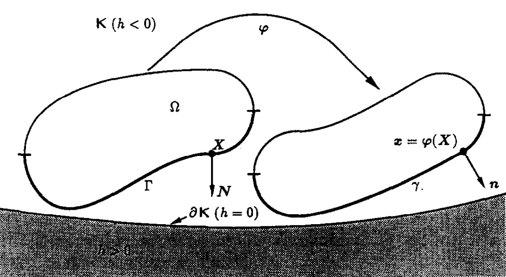
Define a scalar-valued gauge function $h$ satisfying \begin{align} &h<0\quad\text{in }\mathbb{K}\\ &h=0\quad\text{on }\partial\mathbb{K}\\ &h>0\quad\text{outside }\mathbb{K}, \end{align} and for simplicity, it is initially assumed that $\mathbb{K}$ is convex, although this is not a necessary restriction. The contact conditions can, therefore, be stated as follows:

For all $\pmb{X}\in\Gamma$, the admissible deformation $\pmb{x}=\varphi(\pmb{X},t)$ satisfies: \begin{align} &h(\pmb{x})\leq0; \tag{16} \label{eq16}\\ &t_N=-\pmb{n}(\pmb{x})\cdot\pmb{PN}\geq0; \tag{17} \label{eq17}\\ &t_N(\pmb{x})h(\pmb{x})=0; \tag{18} \label{eq18}\\ &\pmb{t}_T=\pmb{PN}+t_N\pmb{n}=\pmb{0}, \tag{19} \label{eq19} \end{align}

where $\pmb{P}$ is the first Piola-Kirchhoff stress tensor , $\pmb{n}$ and $\pmb{N}$ represent the outward normal in the current and reference configuration, respectively. Further explanations regarding the above equations are needed. Equation $\eqref{eq16}$ represents the impermeability of the rigid obstacle to the investigated body; Equation $\eqref{eq17}$ indicates that the surface traction should be compressive; Equation $\eqref{eq18}$ is a contact-detection condition ensuring $t_N\neq0$ only when $h(\pmb{x})=0$; and the frictionless contact is ensured by Equation $\eqref{eq19}$.

It can be seen that Equations $\eqref{eq16}$-$\eqref{eq18}$ are exactly in the same form as the ‘Constraint’, ‘Non-negativity’, and ‘Complementarity’ conditions in the Kuhn-Tucker conditions (see the last three equations $\eqref{eq15}$). Further theoretical details related to contact mechanics will be added to this blog in the future when time permits.

#optimization #contact mechanics

Last modified on 2025-04-22