Preface #
Gradient descent is a first-order iterative algorithm widely used for unconstrained mathematical optimization. It plays a key role in training machine learning models and neural networks, highlighting the importance of the “gradient” in these fields. Generally, there are four approaches to compute the gradient of a certain function: (a) Manual Differentiation, (b) Numerical Differentiation, (c) Symbolic Differentiation, and (d) Automatic Differentiation. In this blog, we will cover the basics, pros, and cons of these four approaches, with the goal of gaining a deeper and more systematic understanding through this organization.
For detailed information, one can refer to the paper Automatic differentiation in machine learning: a survey .
Manual Differentiation #
For a given differentiable function, manual differentiation involves applying basic rules of differentiation (such as power rule, constant rule, sum rule, product rule, quotient rule, and chain rule) to find the rate of change of a function with respect to one of its variables.
When functions become more complicated, manual differentiation is time consuming and prone to error.
Numerical Differentiation #
Numerical differentiation is the process of approximating derivatives using finite differences, based on the values of the original function evaluated at specific sample points. According to the limit definition of a derivative, the gradient of a multivariate function $f: \mathbb{R}^n\to\mathbb{R}$ can be approximated by
$$\frac{\partial f(\pmb{x})}{\partial x_i}\approx\frac{f(\pmb{x}+h\pmb{e}_i)-f(\pmb{x})}{h}, \tag{1} \label{eq1}$$
where $h$ denotes the step size and $\pmb{e}_i$ is the $i$-th unit vector corresponding to variable $x_i$. Equation $\eqref{eq1}$ is also known as the forward difference approximation.
Numerical approximations of derivatives are inherently ill-conditioned and unstable, with the exception of complex variable methods that are applicable to a limited set of holomorphic functions.
--- Bengt Fornberg
Here, the term ill-conditioned and unstable refers to two cardinal sins in numerical analysis: “thou shalt not add small numbers to big numbers”, and “thou shalt not subtract numbers which are approximately equal”. The truncation and round-off errors should be responsible for the drawbacks of numerical approximation. Truncation error approaches zero as $h\to 0$. However, as $h$ decreases, round-off error increases and eventually becomes the dominant factor.
The center difference approximation is employed to partially mitigate the aforementioned errors:
$$\frac{\partial f(\pmb{x})}{\partial x_i}=\frac{f(\pmb{x}+h\pmb{e}_i)-f(\pmb{x}-h\pmb{e}_i)}{2h}+O(h^2), \tag{2} \label{eq2}$$
this method provides an approximation with $O(h^2)$ accuracy, which is one order higher than Equation $\eqref{eq1}$. However, it does not avoid either of the cardinal sins and remains highly inaccurate due to truncation.
Numerical differentiation is not difficult to implement, but the main obstacle to its application lies in the $\mathcal{O}(n)$ time complexity
associated with evaluating $\nabla f$ in $n$ dimensional space. In the field of ML, $n$ can reach millions or even billions in the state-of-the-art deep learning models, making it increasingly challenging for practical use. In contrast, approximation errors are generally tolerated in a deep learning setting due to the well-documented error resiliency of neural network architectures.
Symbolic Differentiation #
Symbolic differentiation is the automatic manipulation of mathematical expressions to obtain derivative expressions. It involves systematically applying the rules of differentiation (like the power rule, product rule, chain rule, etc.) to generate a new symbolic expression that represents the derivative of the original function.
The investigated function (closed-form expression
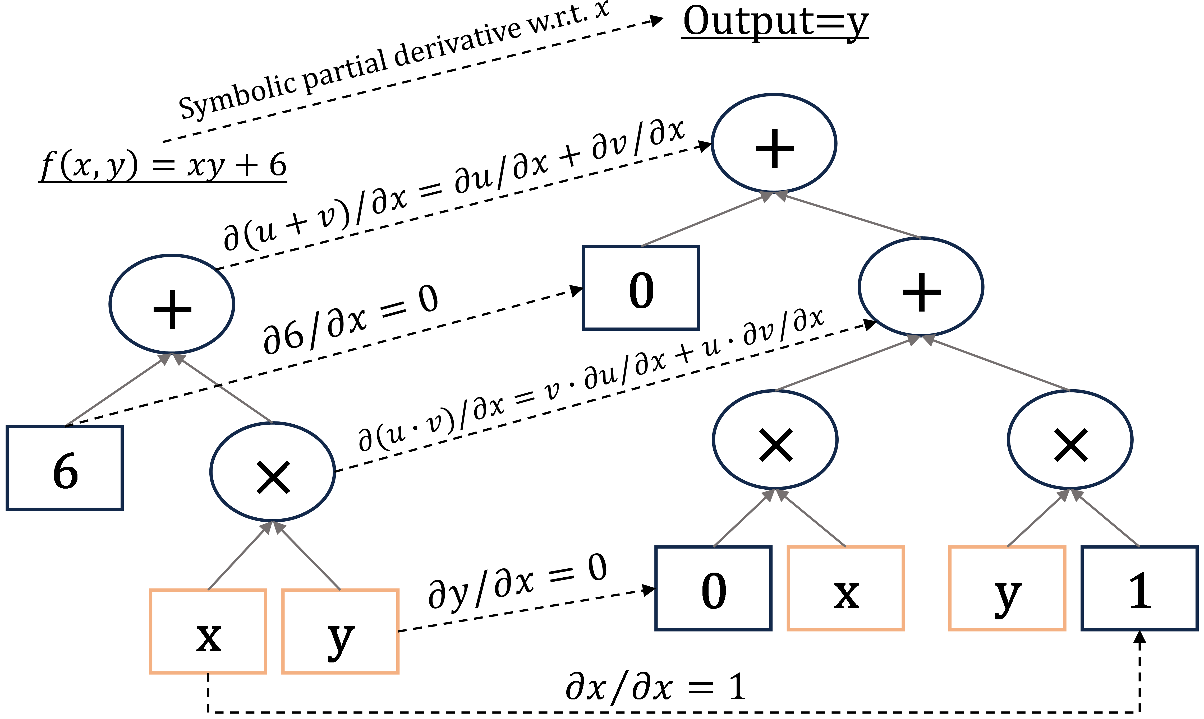
) can be decomposed into a sequence of elementary arithmetic operations (addition, multiplication, etc.) and elementary functions. With basic rules of differentiation (like chain rule, etc.), partial derivatives of each elementary part with respect to a specific variable can be symbolically represented, as shown in Fig. 1.
Figure 1: The process of symbolic differentiation of function f(x,y)=xy+6, this figure shows the partial derivative with respect to variable x.

- Pros: In optimization, symbolic derivatives offer valuable insights into the structure of the problem domain. In certain cases, they can yield analytical solutions for extrema (e.g., like solving
$f^\prime (x)=0$), eliminating the need for numerical derivative calculations entirely. - Cons: It faces the difficulty of translating a computer program into a single mathematical expression, often resulting in inefficient code. Symbolic derivatives can grow exponentially in size compared to the original expression they represent, leading to increased complexity (known as expression swell).
Automatic Differentiation (AD) #
Both classical methods — whether numerical or symbolic — face challenges when computing higher derivatives, as complexity and errors increase. And they tend to be slow when computing partial derivatives w.r.t. multiple inputs, which is essential for gradient-based optimization algorithms. AD solves all of these problems.
All numerical computations are ultimately compositions of a finite set of elementary operations for which derivatives are known. AD refers to a specific family of techniques that compute derivatives through accumulation of (intermediate) values during code execution to generate numerical derivative evaluations rather than derivative expressions. This allows accurate evaluation of derivatives at machine precision with only a small constant factor of overhead and ideal asymptotic efficiency.
--- By this paper
AD can differentiate not only closed-form expressions in classical sense, but also algorithms involve control flow constructs such as braching, loops, recursion, and procedure calls, giving it a significant advantage over symbolic differentiation. AD is blind to any operations, including control flow statements, that do not directly affect numeric values (input, intermediate, output).
There are two primary ways that AD is typically implemented: forward mode and reverse mode.
Forward Accumulation Mode #
In forward mode AD, the process begins by fixing the independent variable w.r.t. which differentiation is performed, and then recursively computing the derivatives of each sub-expression. A typical forward mode AD example is the representation of computing
Figure 2: Evaluation trace of forward primal and forward derivative w.r.t. x1. (Baydin et al., 2018).
$y=f(x_1,x_2)=ln(x_1)+x_1x_2-\sin(x_2)$ as an evaluation trace of elementary operations shown in Fig. 2.

When computing the Jacobian of a function $f: \mathbb{R}^n\to\mathbb{R}^m$ with $n$ independent variables $x_i$ and $m$ dependent outputs $y_j$, each forward pass of AD can be initialized as setting $\dot{\pmb{x}}=\pmb{e}_i$, where $\pmb{e}_i$ is the $i$-th unit vector. Running the code with specific inputs $\pmb{x}=\pmb{a}$ gives one column of the Jacobian
$$\dot{y}_j=\left.\frac{\partial y_j}{\partial x_i}\right|_{\pmb{x}=\pmb{a}},\quad j=1,\cdots,m.$$
Additionally, by initializing with $\dot{\pmb{x}}=\pmb{r}$, one can compute Jacobian-vector products in an efficient and matrix-free manner using forward mode AD
$$\mathrm{\pmb{J}}_f\pmb{r}=\left[\frac{\partial y_i}{\partial x_j}\right]\left\{\pmb{r}\right\}_{n\times 1},\quad i=1,\cdots,m,\ j=1,\cdots,n. \tag{3} \label{eq3}$$
Forward mode AD is efficient and straightforward for functions $f: \mathbb{R}\to\mathbb{R}^m$, as all derivatives $\frac{\mathrm{d}y_i}{\mathrm{d}x}$ can be computed in a single forward pass. Conversely, for functions $f: \mathbb{R}^n\to\mathbb{R}$, forward mode AD requires $n$ evaluations to compute the gradient
$$\nabla f=\left(\frac{\partial y}{\partial x_1},\cdots,\frac{\partial y}{\partial x_n}\right).$$
In summary, for cases $f: \mathbb{R}^n\to\mathbb{R}^m$ where $n\gg m$, a different technique known as the reverse accumulation mode
is often preferred.
Dual Numbers #
Mathematically, forward mode AD can be understood from the perspective of dual numbers
, which are a hypercomplex number system defined as truncated Taylor series: $v+\dot{v}\epsilon$. Here $v, \dot{v}\in\mathbb{R}$ and $\epsilon$ is a nilpotent number satisfying $\epsilon^2=0, \epsilon\neq 0$. In this way, we have
\begin{align} (v+\dot{v}\epsilon)+(u+\dot{u}\epsilon)&=(v+u)+(\dot{v}+\dot{u})\epsilon;\\ (v+\dot{v}\epsilon)(u+\dot{u}\epsilon)&=(vu)+(v\dot{u}+\dot{v}u)\epsilon, \end{align}
note that, the coefficients of $\epsilon$ exactly correspond to the symbolic differentiation rules. Any polynomial $P(x)=p_0+p_1x+\cdots+p_nx^n$ with real coefficients can be extended to a function of a dual-number-valued argument
\begin{align}P(v+\dot{v}\epsilon)&=p_0+p_1v+\cdots+p_nv^n+p_1\dot{v}\epsilon+2p_2v\dot{v}\epsilon+\cdots+np_nv^{n-1}\dot{v}\epsilon\\ &=P(v)+P^\prime(v)\dot{v}\epsilon, \end{align}
where $P^\prime$ is the derivative of $P$. More generally, any (analytic) real function can be extended to dual numbers via its Taylor series expansion
$$f(v+\dot{v}\epsilon)=\sum_{n=0}^\infty\frac{f^{(n)}(v)\dot{v}^n\epsilon^n}{n!}=f(v)+f^\prime(v)\dot{v}\epsilon. \tag{4} \label{eq4}$$
The chain rule works as expected on composite functions based on Equation
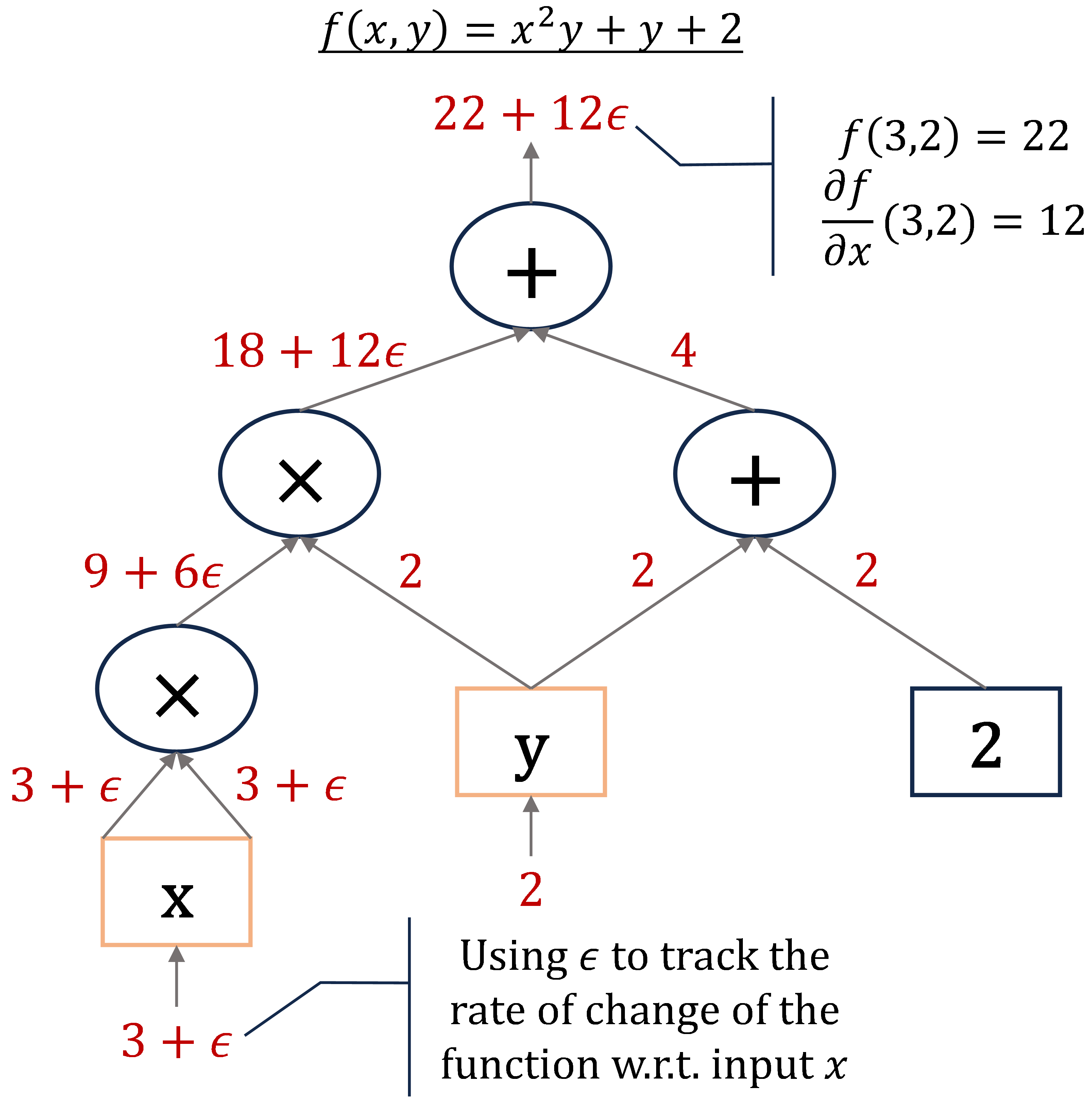
Figure 3: Forward mode autodiff implementation through dual numbers.
$\eqref{eq4}$
$$f(g(v+\dot{v}\epsilon))=f(g(v))+f^\prime(g(v))g^\prime(v)\dot{v}\epsilon,$$
this equation indicates that we can actually extract the derivative of a function by interpreting any non-dual number $v$ as $v+0\epsilon$ and evaluating the function in this non-standard way with an initial input, using a coefficient 1 for $\epsilon$:
$$\left.\frac{\mathrm{d}f(x)}{\mathrm{d}x}\right|_{x=v}=\mathrm{epsilon\ coefficient}\left(f(v+1\cdot\epsilon)\right),$$
one can refer to the example shown in Fig. 3, which illustrates the computation of the partial derivative $\partial f/\partial x$ at point $(3,2)$.

The perspective of dual number enables the simultaneous computation of both the function and its derivative.
Reverse Accumulation Mode #
Reverse accumulation mode (generalized backpropagation algorithm) computes the gradients of a function w.r.t. its inputs by first evaluating the function and then backpropagating the gradients through the computation graph in reverse order. This mode is particularly efficient when there are many inputs but relatively few outputs, i.e., $n\gg m$ (as is often the case in machine learning, especially for loss functions and neural networks).
In this mode, the quantity of interest is termed as an “adjoint”, which represents the sensitivity of a considered dependent variable $y_j$ w.r.t. changes in $v_i$
$$\bar{v}_i=\frac{\partial y_j}{\partial v_i}=\sum_{j\in\left\{\mathrm{successors\ of\ i}\right\}}\bar{v}_j\frac{\partial v_j}{\partial v_i},$$
moreover, for backpropagation, $y$ should be a scalar corresponding to the network error.
So how exactly does reverse accumulation work? The corresponding two-step process is outlined below:
- (Function Evaluation) The original function code is run forward, populating intermediate variables
$v_i$and recording the dependencies in the computational graph through a bookkeeping procedure; - (Gradient Computation) Derivatives are calculated by propagating adjoints
$\bar{v}_i$in reverse, from the outputs back to the inputs.
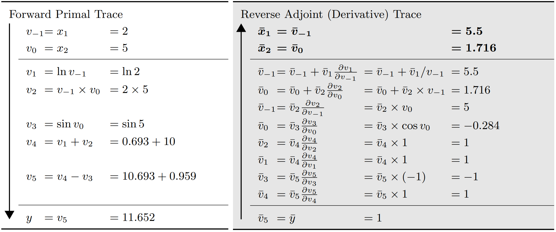
An example of reverse mode AD can be found in Fig. 4, where the function and derivative values of
Figure 4: Evaluation trace of forward primal and reverse adjoint derivative (Baydin et al., 2018).
$y=f(x_1,x_2)=ln(x_1)+x_1x_2-\sin(x_2)$ are obtained through both a forward and a backward pass. Taking the node $v_0$ as an example, it can only affect the final output through affecting $v_2$ and $v_3$, so its adjoint $\bar{v}_0$ is given by
$$\frac{\partial y}{\partial v_0}=\frac{\partial y}{\partial v_2}\frac{\partial v_2}{\partial v_0}+\frac{\partial y}{\partial v_3}\frac{\partial v_3}{\partial v_0}.$$

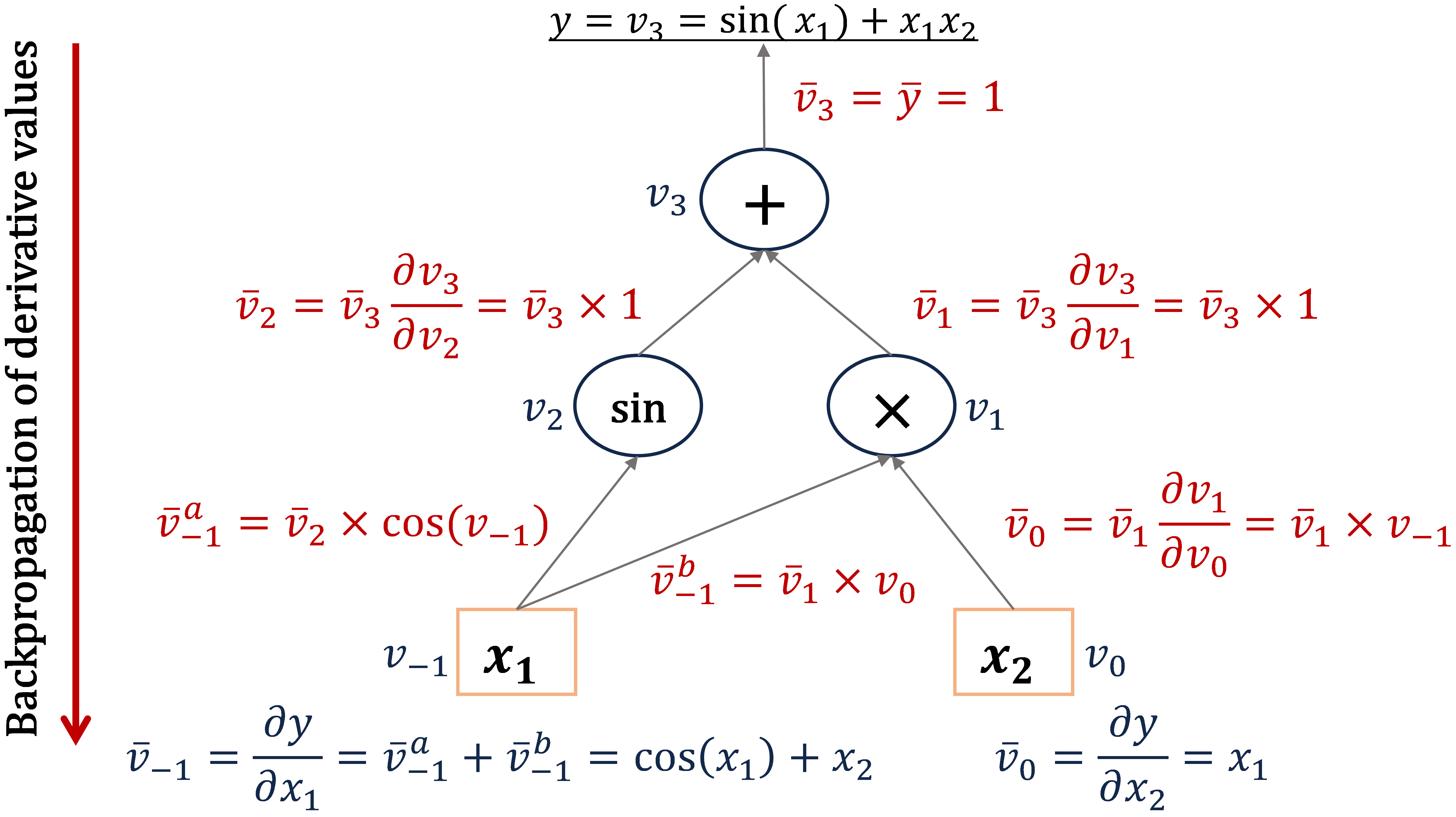
Here, we also present an intuitive illustration of how reverse mode AD compute the partial derivatives of function
Figure 5: Computational graph of reverse accumulation mode AD.
$y=\sin(x_1)+x_1x_2$ through backpropagation (see Fig. 5).

Similar to the matrix-free computation of Jacobian-vector product with forward mode AD (Equation $\eqref{eq3}$), by initializing the reverse phase with $\bar{\pmb{y}}=\pmb{r}$, the reverse one can be used for computing the transposed Jacobian-vector product
$$\mathrm{\pmb{J}}_f^\mathrm{T}\pmb{r}=\left[\frac{\partial y_j}{\partial x_i}\right]\left\{\pmb{r}\right\}_{m\times 1},\quad i=1,\cdots,n,\ j=1,\cdots,m.$$
One more point to note is that the advantages of reverse mode AD come at the cost of increased storage requirements, which can grow in proportion to the number of operations in the evaluated function.
#machine learningLast modified on 2026-01-08