Variational Diffusion Models (VDMs = MHVAE + 3 Restrictions) #
A VDM can be viewed as a Markovian Hierarchical VAE plus three key restrictions:
- The latent dimension is exactly equal to the data dimension
- The structure of the latent encoder at each timestep is not learned; it is pre-defined as a linear Gaussian model. In other words, it is a Gaussian distribution centered around the output of the previous timestep
- The Gaussian parameters of the latent encoders vary over time in such a way that the distribution of the latent at final timestep
$T$is a standard Gaussian
The Markov property between hierarchical transitions from a standard MHVAE is explicitly maintained. We then present related explanations of the above assumptions.
The first restriction: with some abuse of notation, both true data sample and latent variables can be represented as $\pmb{x}_t$, in this way, $t=0$ denotes true data samples and $t\in\left[1,T\right]$ denotes a corresponding latent with hierarchy $t$. The VDM posterior can be re-expressed in a form similar to the MHVAE posterior (see Equation (7) in this Blog
):
$$q(\pmb{x}_{1:T}|\pmb{x}_0)=\prod_{t=1}^Tq(\pmb{x}_t|\pmb{x}_{t-1})$$
The second restriction pre-defined the distribution of each latent variable in the encoder to be a Gaussian centered around its previous hierarchical latent. Unlike a MHVAE, the structure of the encoder at each timestep is not learned, it is fixed as a linear Gaussian model, where the mean and standard deviation can be set beforehand as hyperparameters or learned as parameters.
We choose to parameterize the Gaussian encoder with mean $\pmb{\mu}_t(\pmb{x}_t)=\sqrt{\alpha_t}\pmb{x}_{t-1}$, and variance $\sum_t(\pmb{x}_t)=(1-\alpha_t)\pmb{\mathrm{I}}$. The coefficient forms are chosen such that the variance of the latent variables stay at a similar scale; alternatively, the encoding process is variance-preserving. The main takeaway is that $\alpha_t$ is a (potentially learnable) coefficient that can vary with the hierarchical depth $t$ for flexibility. The encoder transitions are mathematically denoted as:
$$q(\pmb{x}_t|\pmb{x}_{t-1})=\mathcal{N}(\pmb{x}_t; \sqrt{\alpha_t}\pmb{x}_{t-1},(1-\alpha_t)\pmb{\mathrm{I}})$$
The third restriction indicates that $\alpha_t$ evolves over time according to a fixed or learnable schedule structured such that the distribution of the final latent $p(\pmb{x}_T)$ is a standard Gaussian. The joint distribution for a VDM can be updated based on that of a MHVAE (see Equation (6) in this Blog
):
$$p(\pmb{x}_{0:T})=p(\pmb{x}_T)\prod_{t=1}^Tp_{\pmb{\theta}}(\pmb{x}_{t-1}|\pmb{x}_t),\quad\text{where, }p(\pmb{x}_T)=\mathcal{N}(\pmb{x}_T; \pmb{0}, \pmb{\mathrm{I}}),$$
note that, the property of Markov chain is adopted: $p(\pmb{x}_{0:T})=p(\pmb{x}_T)p(\pmb{x}_{0:T-1}|\pmb{x}_T)=p(\pmb{x}_T)p(\pmb{x}_{T-1}|\pmb{x}_T)p(\pmb{x}_{0:T-2}|\pmb{x}_{T-1},\pmb{x}_T)\stackrel{Markov Chain}{\longrightarrow}p(\pmb{x}_{0:T-2}|\pmb{x}_{T-1})$
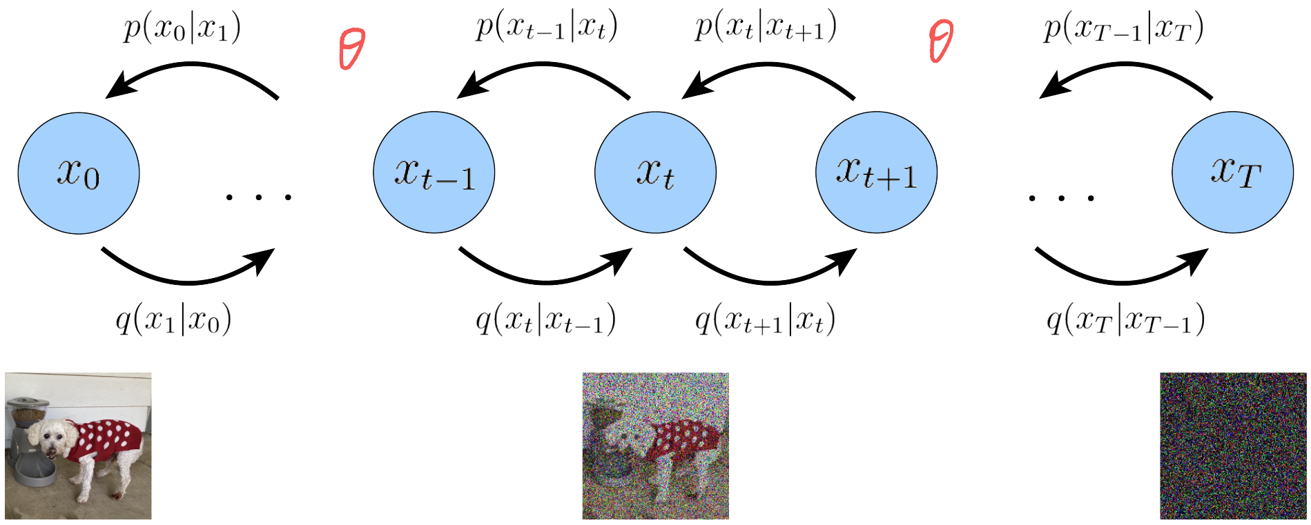
These three restrictions collectively describe a steady noisification of an image input over time, we progressively corrupt an image by adding Gaussian noise until eventually it becomes completely identical to pure Gaussian noise. This is illustrated in Fig. 1.
Figure 1: A visual representation of a VDM. Each encoding process is modeled as a Gaussian distribution that uses the output of the previous state as its mean (Calvin Luo, 2022).

The subsequent interpretations of each ELBO term of a VDM will not be given in detail due to the lengthy derivations, but you can refer to some notes I made on the paper Understanding Diffusion Models: A Unified Perspective, which is given below
The Main Takeaway #
We have therefore derived three equivalent objectives to optimize a VDM:
- learning a neural network to predict the original image
$\pmb{x}_0$(the ground truth); - the source noise
$\pmb{\epsilon}_0\sim\mathcal{N}(\pmb{\epsilon}; \pmb{0}, \pmb{\mathrm{I}})$. Empirically, some works have found that predicting the noise resulted in better performance; - or the score of the image at an arbitrary noise level
$\nabla log\,p(\pmb{x}_t)$.
The VDM can be scalably trained by stochastically sampling timesteps $t$ and minimizing the norm of the prediction with the ground truth target.
Last modified on 2026-01-08