Variational Autoencoders (VAEs) #
Dissecting the ELBO #
This approach is “variational” because we optimize for the best $q_{\pmb{\phi}}(\pmb{z}|\pmb{x})$ amongst a family of potential posterior distributions parameterized by $\pmb{\phi}$; it is called “autoencoder” due to its resemblance to a traditional autoencoder model, where input data is trained to predict itself after undergoing an intermediate bottlenecking representation step. Dissecting the ELBO term:
\begin{align} \mathbb{E}_{q_{\pmb{\phi}}(\pmb{z}|\pmb{x})}\left[log\frac{p(\pmb{x}, \pmb{z})}{q_{\pmb{\phi}}(\pmb{z}|\pmb{x})}\right] &= \mathbb{E}_{q_{\pmb{\phi}}(\pmb{z}|\pmb{x})}\left[log\frac{p_{\pmb{\theta}}(\pmb{x}|\pmb{z})p(\pmb{z})}{q_{\pmb{\phi}}(\pmb{z}|\pmb{x})}\right] \tag{1}\\ &= \mathbb{E}_{q_{\pmb{\phi}}(\pmb{z}|\pmb{x})}\left[log\,p_{\pmb{\theta}}(\pmb{x}|\pmb{z})\right]+\mathbb{E}_{q_{\pmb{\phi}}(\pmb{z}|\pmb{x})}\left[log\frac{p(\pmb{z})}{q_{\pmb{\phi}}(\pmb{z}|\pmb{x})}\right] \tag{2}\\ &= \underbrace{\mathbb{E}_{q_{\pmb{\phi}}(\pmb{z}|\pmb{x})}\left[log\,p_{\pmb{\theta}}(\pmb{x}|\pmb{z})\right]}_{\text{reconstruction term}}-\underbrace{D_{\mathrm{KL}}\left(q_{\pmb{\phi}}(\pmb{z}|\pmb{x})\|p(\pmb{z})\right)}_{\text{prior matching term}} \tag{3} \label{eq3} \end{align}
From the derivation, we know that there are two main steps for the learning process:
- Learn an intermediate bottlenecking distribution
$q_{\pmb{\phi}}(\pmb{z}|\pmb{x})$that can be treated as an encoder, which transforms inputs into a distribution over possible latents. - Learn a deterministic function
$p_{\pmb{\theta}}(\pmb{x}|\pmb{z})$to convert a given latent vector$\pmb{z}$into an observation$\pmb{x}$, which can be interpreted as a decoder.
We also present some necessary comments regarding Equation $\eqref{eq3}$:
- The first term measures the reconstruction likelihood of the decoder from our variational distribution; this ensures that the learned distribution is modeling effective latents that the original data can be regenerated from.
- The second term measures how similar the learned variational distribution is to a prior belief held over latent variables.
Maximizing the ELBO is thus equivalent to maximizing its first term and minimizing its second term.
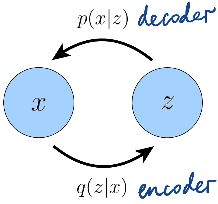
A graphic representation can be seen in the figure below:
Figure 1: Representation of basic encoder-decoder process in VAEs (Calvin Luo, 2022).

A defining feature of the VAE is how the ELBO is optimized jointly over parameters $\pmb{\phi}$ and $\pmb{\theta}$. The encoder of the VAE is generally chosen to model a multivariate Gaussian with diagonal covariance, and the prior is often a standard multivariate Gaussian:
\begin{align} q_{\pmb{\phi}}(\pmb{z}|\pmb{x}) &= \mathcal{N}\left(\pmb{z};\pmb{\mu}_{\pmb{\phi}}(\pmb{x}),\pmb{\sigma_{\phi}}^2(\pmb{x})\pmb{\mathrm{I}}\right) \tag{4}\\ p(\pmb{z}) &= \mathcal{N}\left(\pmb{z};\pmb{0},\pmb{\mathrm{I}}\right), \tag{5} \end{align}
with this kind of settings, the prior matching term of the ELBO (Equation $\eqref{eq3}$) can be computed analytically, and the reconstruction term can be approximated using a Monte Carlo estimate. We now rewrite our objective:

The latents $\left\lbrace\pmb{z}^{(l)}\right\rbrace_{l=1}^L$ are sampled from $q_{\pmb{\phi}}(\pmb{z}|\pmb{x})$ for every observation $\pmb{x}$ in the dataset. Note that there arises a problem: each $\pmb{z}^{(l)}$ that our loss is computed on is generated by a stochastic sampling procedure, which is generally non-differentiable. Fortunately, it can be addressed when $q_{\pmb{\phi}}(\pmb{z}|\pmb{x})$ is pre-designed to model certain distributions like multivariate Gaussian. This is called the reparameterization trick.
Reparameterization Trick #
In this approach, a random variable is rewritten as a deterministic function of a noise variable, which allows for the optimization of the non-stochastic terms through gradient descent. For example, samples from a normal distribution $x\sim\mathcal{N}(x;\mu,\sigma^2)$ with arbitrary mean $\mu$ and variance $\sigma^2$ can be reparameterized as:
$$x=\mu+\sigma\epsilon\quad\text{with }\epsilon\sim\mathcal{N}(\epsilon;0,\mathrm{I}),$$
which means, by the reparameterization trick, sampling from an arbitrary Gaussian distribution can be performed by sampling from a standard Gaussian, scaling the result by the target standard deviation, and shifting it by the target mean.
In VAEs, each $\pmb{z}$ is computed as a deterministic function of input $\pmb{x}$ and auxiliary noise variable $\pmb{\epsilon}$:
$$\pmb{z}=\pmb{\mu}_{\pmb{\phi}}(\pmb{x})+\pmb{\sigma}_{\pmb{\phi}}(\pmb{x})\otimes\pmb{\epsilon}\quad\text{with }\pmb{\epsilon}\sim\mathcal{N}(\pmb{\epsilon};\pmb{0}, \pmb{\mathrm{I}}),$$
here $\otimes$ denotes an element-wise product. In this way, gradients can then be computed w.r.t. $\pmb{\phi}$ to thus optimize $\pmb{\mu}_{\pmb{\phi}}$ and $\pmb{\sigma}_{\pmb{\phi}}$. The VAE actually utilizes the reparameterization and Monte Carlo estimates to optimize the ELBO jointly over $\pmb{\phi}$ and $\pmb{\theta}$.
Once a VAE trained, generating new data can be performed by sampling directly from the latent space $p(\pmb{z})$ and then running it through the decoder.
VAEs are particularly interesting when the dimensionality of $\pmb{z}$ is less than that of input $\pmb{x}$, as we might then be learning compact, useful representations. Furthermore, when a semantically meaningful latent space is learned, latent vectors can be edited before being passed to the decoder to more precisely control the data generated.
Hierarchical Variational Autoencoders (HVAEs) #
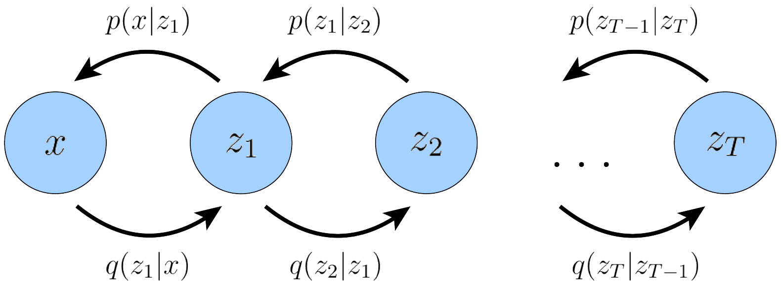
HVAE — a generalization of a VAE that extends to multiple hierarchies over latent variables. Under this formulation, latent variables themselves are interpreted as generated from other higher-level, more abstract latents.
Whereas in the general HVAE with
Figure 2: A MHVAE with T hierarchical latents (Calvin Luo, 2022).
$T$ hierarchical levels, each latent is allowed to condition on all previous latents, here we focus on a special case which we call a Markovian HVAE (MHVAE). In a MHVAE, the generative process is a Markov chain; that is, each transition down the hierarchy is Markovian, where decoding each latent $\pmb{z}_t$ only conditions on previous latent $\pmb{z}_{t+1}$, as shown in Fig. 2.

The joint distribution and the posterior of a Markovian HVAE can be represented as:
\begin{align} p(\pmb{x}, \pmb{z}_{1:T})&=p(\pmb{z}_T)p_{\pmb{\theta}}(\pmb{x}|\pmb{z}_t)\prod_{t=2}^T p_{\pmb{\theta}}(\pmb{z}_{t-1}|\pmb{z}_t) \tag{6}\label{eq6}\\ q_{\pmb{\phi}}(\pmb{z}_{1:T}|\pmb{x})&=q_{\pmb{\phi}}(\pmb{z}_1|\pmb{x})\prod_{t=2}^Tq_{\pmb{\phi}}(\pmb{z}_t|\pmb{z}_{t-1}) \tag{7}\label{eq7} \end{align}
The ELBO can be readily extended to the case of hierarchical VAEs:
\begin{align} log\,p(\pmb{x}) &= log\int p(\pmb{x}, \pmb{z}_{1:T})\,\mathrm{d}\pmb{z}_{1:T}\\ &= log\int\frac{p(\pmb{x}, \pmb{z}_{1:T})q_{\pmb{\phi}}(\pmb{z}_{1:T}|\pmb{x})}{q_{\pmb{\phi}}(\pmb{z}_{1:T}|\pmb{x})}\,\mathrm{d}\pmb{z}_{1:T}\\ &= log\mathbb{E}_{q_{\pmb{\phi}}(\pmb{z}_{1:T}|\pmb{x})}\left[\frac{p(\pmb{x}, \pmb{z}_{1:T})}{q_{\pmb{\phi}}(\pmb{z}_{1:T}|\pmb{x})}\right]\\ &\geq\mathbb{E}_{q_{\pmb{\phi}}(\pmb{z}_{1:T}|\pmb{x})}\left[log\frac{p(\pmb{x}, \pmb{z}_{1:T})}{q_{\pmb{\phi}}(\pmb{z}_{1:T}|\pmb{x})}\right]. \tag{8}\label{eq8} \end{align}
With the joint distribution (Equation $\eqref{eq6}$) and posterior (Equation $\eqref{eq7}$), the right hand side of Equation $\eqref{eq8}$ is re-expressed as:
$$\mathbb{E}_{q_{\pmb{\phi}}(\pmb{z}_{1:T}|\pmb{x})}\left[log\frac{p(\pmb{x}, \pmb{z}_{1:T})}{q_{\pmb{\phi}}(\pmb{z}_{1:T}|\pmb{x})}\right]=\mathbb{E}_{q_{\pmb{\phi}}(\pmb{z}_{1:T}|\pmb{x})}\left[log\frac{p(\pmb{z}_T)p_{\pmb{\theta}}(\pmb{x}|\pmb{z}_t)\prod_{t=2}^T p_{\pmb{\theta}}(\pmb{z}_{t-1}|\pmb{z}_t)}{q_{\pmb{\phi}}(\pmb{z}_1|\pmb{x})\prod_{t=2}^Tq_{\pmb{\phi}}(\pmb{z}_t|\pmb{z}_{t-1})}\right],$$
which is the MHVAE ELBO.
Last modified on 2026-01-08